In NLP domian, the Transformer from the 2017 paper “Attention is All You Need” has been on a lot of people’s minds over the last few years. Besides producing major improvements in translation quality, it provides a new architecture for many other NLP tasks. The paper itself is very clearly written, but the conventional wisdom has been that it is quite difficult to implement correctly.
ArXiv Link:
https://arxiv.org/abs/1706.03762
From: Ashish Vaswani [view email]
[v1] Mon, 12 Jun 2017 17:57:34 UTC (1,102 KB)
[v2] Mon, 19 Jun 2017 16:49:45 UTC (1,125 KB)
[v3] Tue, 20 Jun 2017 05:20:02 UTC (1,125 KB)
[v4] Fri, 30 Jun 2017 17:29:30 UTC (1,124 KB)
[v5] Wed, 6 Dec 2017 03:30:32 UTC (1,124 KB)[v5] Wed, 6 Dec 2017 03:30:32 UTC (1,124 KB)
In this post I present an “annotated” version of the paper in the form of a line-by-line implementation to build an English-to-Chinese translator. I have reordered and deleted some sections from the original paper and also added comments/figures and explanations throughout the post to keep model structure clear and the code block more meaningful.
To follow along, you are required t know neural networks and word embedding, and Python and familiar with PyTorch package and Nvidia CUDA drives.
The document images and styles are inspired by The Illustrated Transformer from Jay Alammer. The code here is based heavily on harverdnlp : The Annotated Transformer. The English-to-Chinese translator project is based on my NLP training camp from GreedAI Course.
Project: English-Chinese Translator
The original Harvard NLP blog applied the English- to-German translation task, but I adapted it to the English- to-Chinese translation task in this work.
In this post, we will build a Transformer model to translate English sentence to Chinese sentences with PyTorch instead of applying the popular Hugging-face packages. The data set is a small set including around 10k sentence for training which is sufficient for learning and get the basic job done. If you are looking for better performance, large data set are required and you will need GPU support to reduce the training time.
GitHub Repository: Annotated-Transformer-English-to-Chinese-Translator .
Notification: Before reading the code, please review the PyTorch nn.model frameworks WHAT IS TORCH.NN REALLY.
1. Understand the Transformer Model
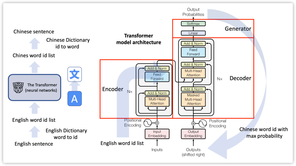
First of all, Transformer is a neural network model or deep networks model with encoder-decoder structure, special layer design (i.e., multi-head self-attention layer) and connections. Moreover, the Transformer is the first transduction model relying entirely on self-attention to compute representations of its input and output without using sequence aligned RNNs or convolution.
A High-Level Look
Let’s look at the Transformer model as a single black box. In a machine translation application, it would take a sentence in one language, and output its translation in another.
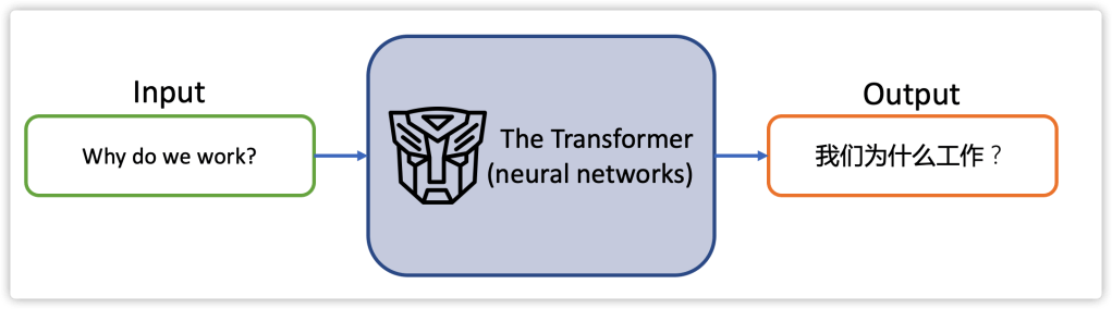
Here is an example from Google Translate:

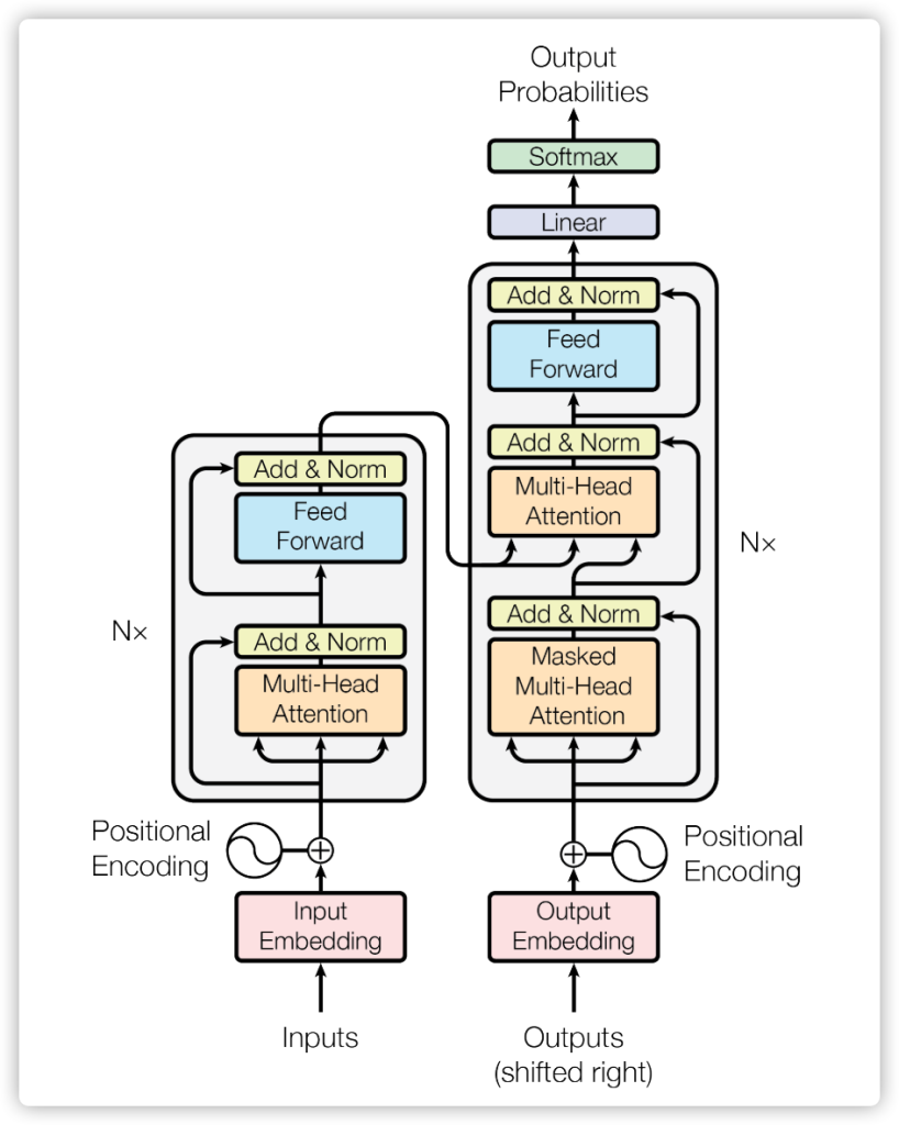
To reveal more details in Fig 03, we open up the Transformer model and see an encoding component, a decoding component, and connections between them. One step further, the encoding component is a stack of encoders (the paper stacks six of them (N=6) on top of each other – there’s nothing magical about the number six, one can definitely experiment with other arrangements). The decoding component is a stack of decoders of the same number.

Understand the Basic Function
Here I will assume you know LSTM (one type of recurrent neural networks) as Fig 04 shows. It is a sequence to sequence model, it has to make prediction iteratively even in training phases. In other words, it is a sequential process.
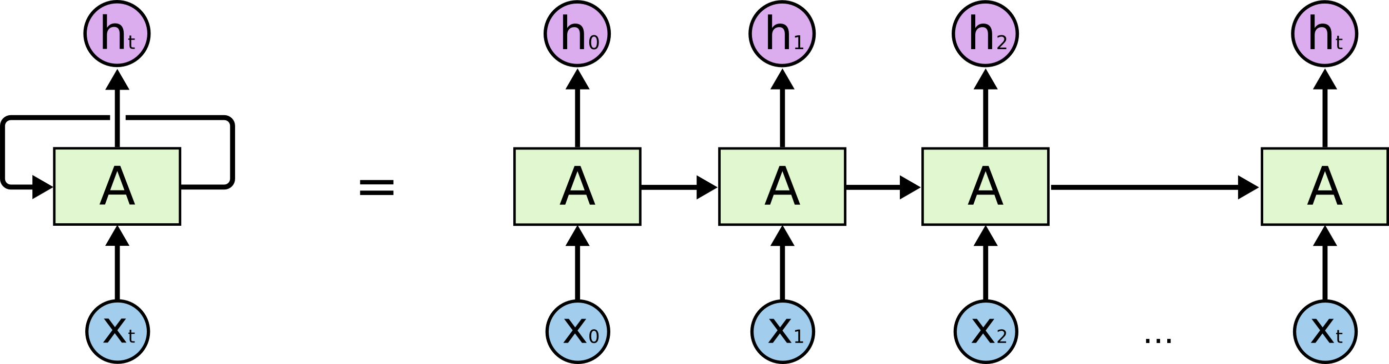
But Transformer is different, it can be trained in parallel fashion take all the input sequence at the same time which boosts the training efficiency. It uses the positional encoding to understand the word order with the help of attention mechanism to understand the context. I will give more details in the following sections.
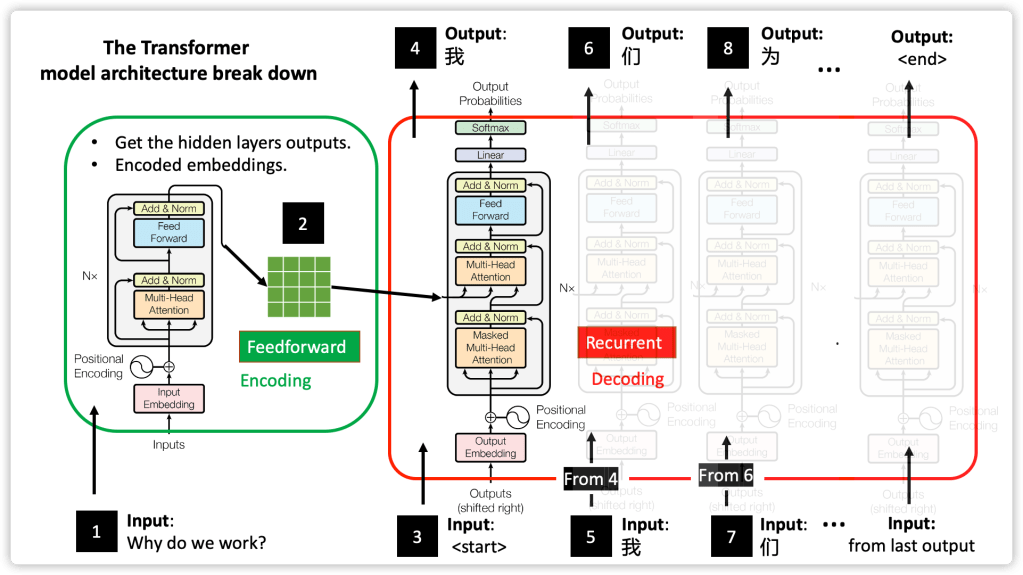
The Whole Transformer encoder-decoder model architecture services for the following purposes.
- Encoder(s): the encoding process transforms the input sentence (list of English words) into numeric matrix format (embedding ), consider this step is to extract useful and necessary information for the decoder. In Fig 06, the embedding is represented by the greed matrix.
- Decoder(s): then the decoding process mapping these embeddings back to another language sequence as Fig 06 shown, which helps us to solve all kinds of supervised NLP tasks, like machine translation (in this blog), sentiment classification, entity recognition, summary generation, semantic relation extraction and so on.
In sum, the encoder maps an input sequence of symbol representations (x1, …, xn) to a sequence of continuous representations z = (z1, …, zn). Given z, the decoder then generates an output sequence (y1, …, ym) of symbols one element at a time. At each step the model is auto-regressive.
2. Encoder
We will focus on the structure of the encoder in this section, because after understanding the structure of the encoder, understanding the decoder will be very simple. Moreover we can just use the encoder to complete some of the mainstream tasks in NLP, such as sentiment classification, semantic relationship analysis, named entity recognition and so on.
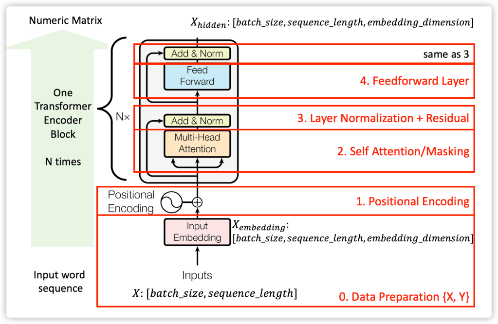
Recall that the Encoder denotes the process of mapping natural language sequences to mathematical expressions to hidden layers outputs.
Let us take a close look at the encoder stacks of Transformer. The the following sections will refer to the 0, 1,2,3,4 blocks: 0. Data preparation (word to numbers / input embedding/batch/masking); 1. Positional Encoding. 2. Self-Attention; 3. Layer Normalisation and Residual Connections. 4. Position-wise Feed-Forward Network.
2.0 Data Preparation: English-to-Chinese Translator Data
The data can be downloaded from here. There are 7 txt files: cmn.txt is the full data set; The train.txt, dev.txt, test.txt are 80% -10%-10% of the full dataset which are the data file to built the Transformer. The train_mini.txt, dev_mini.txt, test_mini.txt are used for debug and learning only contain 1000, 200 and 200 rows, respectively.
| File name | Lines | Ratio | Note |
|---|---|---|---|
| cmt.txt | 18,167 | 100% | Full data set |
| train.txt | 14533 | 80% | Training |
| dev.txt | 1817 | 10% | Validation |
| test.txt | 1817 | 10% | Test |
| train_mini.txt | 1000 | — | — |
| dev_mini.txt | 200 | — | — |
| test_mini.txt | 200 | — | — |
For example, the txt data English and Chinese sentence pairs look like follows:
Hi. 嗨。
Hi. 你好。
Run. 跑。
Wait! 等等!
Hello! 你好。
I try. 让我来。
… …
I think we should talk about this now. 我认为我们现在就该谈谈这个。
I think you should eat a ham sandwich. 我认为你该吃火腿三明治。
… …
Even now, I occasionally think I’d like to see you. Not the you that you are today, but the you I remember from the past. 即使是现在,我偶尔还是想见到你。不是今天的你,而是我记忆中曾经的你。
If a person has not had a chance to acquire his target language by the time he’s an adult, he’s unlikely to be able to reach native speaker level in that language. 如果一個人在成人前沒有機會習得目標語言,他對該語言的認識達到母語者程度的機會是相當小的。
DEBUG MODE
In the following code, we first import all the packages we need, then we set DEBUG variable to control two sets of the hyper-parameters, the first-group is for debug / learning, which makes the code run in 30s. The other one is used for real training setup. As you can see, the DEBUG mode makes all the numbers smaller including the training epoch, encoder and decoder layers, hidden node numbers, and try to build a Transformer model with the mini dataset.
This is quite important for practice in ML/DL model building, always start from a sample set from the large data set.
import os
import math
import copy
import time
import numpy as np
import torch
import torch.nn as nn
import torch.nn.functional as F
from nltk import word_tokenize
from collections import Counter
from torch.autograd import Variable
import seaborn as sns
import matplotlib.pyplot as plt

# init parameters
UNK = 0  # unknow word-id
PAD = 1  # padding word-id
BATCH_SIZE = 64

DEBUG = True    # Debug / Learning Purposes.
# DEBUG = False # Build the model, better with GPU CUDA enabled.

if DEBUG:
    EPOCHS  = 2
    LAYERS  = 3
    H_NUM   = 8
    D_MODEL = 128
    D_FF    = 256
    DROPOUT = 0.1
    MAX_LENGTH = 60
    TRAIN_FILE = 'data/nmt/en-cn/train_mini.txt'
    DEV_FILE   = 'data/nmt/en-cn/dev_mini.txt'
    SAVE_FILE  = 'save/models/model.pt'
else:
    EPOCHS  = 20
    LAYERS  = 6
    H_NUM   = 8
    D_MODEL = 256
    D_FF    = 1024
    DROPOUT = 0.1
    MAX_LENGTH = 60
    TRAIN_FILE = 'data/nmt/en-cn/train.txt'
    DEV_FILE   = 'data/nmt/en-cn/dev.txt'
    SAVE_FILE  = 'save/models/large_model.pt'

DEVICE = torch.device("cuda" if torch.cuda.is_available() else "cpu")
Data PrepRocessing.
The data preprocess contains four steps.
- Load the sentence and tokenize the sentence and add start/end marks(Begin of Sentence /End of Sentence vs BOS/ EOS).
- Build dictionaries including ‘word-to-id’ and inverted dictionary ‘id-to-word’: English and Chinese, ‘word: index}, i.e, {‘english’: 1234}, {1234: ‘english’}.
- Sort the dictionaries to reduce padding.
- Split the dataset into patches for training and validation.
def seq_padding(X, padding=0):
    """
    add padding to a batch data
    """
    L = [len(x) for x in X]
    ML = max(L)
    return np.array([
        np.concatenate([x, [padding] * (ML - len(x))]) if len(x) < ML else x for x in X
    ])

class PrepareData:
    def __init__(self, train_file, dev_file):
        # 01. Read the data and tokenize
        self.train_en, self.train_cn = self.load_data(train_file)
        self.dev_en, self.dev_cn     = self.load_data(dev_file)

        # 02. build dictionary: English and Chinese
        self.en_word_dict, self.en_total_words, self.en_index_dict = self.build_dict(self.train_en)
        self.cn_word_dict, self.cn_total_words, self.cn_index_dict = self.build_dict(self.train_cn)

        # 03. word to id by dictionary Use input word list length to sort, reduce padding
        self.train_en, self.train_cn = self.wordToID(self.train_en, self.train_cn, self.en_word_dict, self.cn_word_dict)
        self.dev_en, self.dev_cn     = self.wordToID(self.dev_en, self.dev_cn, self.en_word_dict, self.cn_word_dict)

        # 04. batch + padding + mask
        self.train_data = self.splitBatch(self.train_en, self.train_cn, BATCH_SIZE)
        self.dev_data   = self.splitBatch(self.dev_en, self.dev_cn, BATCH_SIZE)

    def load_data(self, path):
        """
        Read English and Chinese Data
        tokenize the sentence and add start/end marks(Begin of Sentence; End of Sentence)
        en = [['BOS', 'i', 'love', 'you', 'EOS'],
              ['BOS', 'me', 'too', 'EOS'], ...]
        cn = [['BOS', '我', '爱', '你', 'EOS'],
              ['BOS', '我', '也', '是', 'EOS'], ...]
        """
        en = []
        cn = []
        with open(path, 'r', encoding='utf-8') as f:
            for line in f:
                line = line.strip().split('\t')
                en.append(["BOS"] + word_tokenize(line[0].lower()) + ["EOS"])
                cn.append(["BOS"] + word_tokenize(" ".join([w for w in line[1]])) + ["EOS"])
        return en, cn

    def build_dict(self, sentences, max_words = 50000):
        """
        sentences: list of word list
        build dictonary as {key(word): value(id)}
        """
        word_count = Counter()
        for sentence in sentences:
            for s in sentence:
                word_count[s] += 1

        ls = word_count.most_common(max_words)
        total_words = len(ls) + 2
        word_dict = {w[0]: index + 2 for index, w in enumerate(ls)}
        word_dict['UNK'] = UNK
        word_dict['PAD'] = PAD
        # inverted index: {key(id): value(word)}
        index_dict = {v: k for k, v in word_dict.items()}
        return word_dict, total_words, index_dict

    def wordToID(self, en, cn, en_dict, cn_dict, sort=True):
        """
        convert input/output word lists to id lists.
        Use input word list length to sort, reduce padding.
        """
        length = len(en)
        out_en_ids = [[en_dict.get(w, 0) for w in sent] for sent in en]
        out_cn_ids = [[cn_dict.get(w, 0) for w in sent] for sent in cn]

        def len_argsort(seq):
            """
            get sorted index w.r.t length.
            """
            return sorted(range(len(seq)), key=lambda x: len(seq[x]))

        if sort: # update index
            sorted_index = len_argsort(out_en_ids) # English
            out_en_ids = [out_en_ids[id] for id in sorted_index]
            out_cn_ids = [out_cn_ids[id] for id in sorted_index]
        return out_en_ids, out_cn_ids

    def splitBatch(self, en, cn, batch_size, shuffle=True):
        """
        get data into batches
        """
        idx_list = np.arange(0, len(en), batch_size)
        if shuffle:
            np.random.shuffle(idx_list)

        batch_indexs = []
        for idx in idx_list:
            batch_indexs.append(np.arange(idx, min(idx + batch_size, len(en))))

        batches = []
        for batch_index in batch_indexs:
            batch_en = [en[index] for index in batch_index]
            batch_cn = [cn[index] for index in batch_index]
            # paddings: batch, batch_size, batch_MaxLength
            batch_cn = seq_padding(batch_cn)
            batch_en = seq_padding(batch_en)
            batches.append(Batch(batch_en, batch_cn))
            #!!! 'Batch' Class is called here but defined in later section.
        return batches
Input/Output Embeddings
Similary to all sequential model, we used learned embedding to convert the input/output vectors’ dimensionality to d-model. In our model, the two embedding layers and pre-softmax layer will share weight matrix.
class Embeddings(nn.Module):
    def __init__(self, d_model, vocab):
        super(Embeddings, self).__init__()
        self.lut = nn.Embedding(vocab, d_model)
        self.d_model = d_model

    def forward(self, x):
        # return x's embedding vector(times math.sqrt(d_model))
        return self.lut(x) * math.sqrt(self.d_model)
Now, we have all the code for data preprocessing. Let’s focus on the understand and build Transformer mode.
2.1 Positional Encoding
The Transformer does not contain iteration operation like RNN or LSTM in encoders, so we have to offer the position information of the words to the model, so the model learns the order in the input sequence.
Thus, we define the positional encoding as [max_sequence_length, embedding_dimension]
In the paper, we use sine and cosine function to provide the position information.
class PositionalEncoding(nn.Module):
    def __init__(self, d_model, dropout, max_len=5000):
        super(PositionalEncoding, self).__init__()
        self.dropout = nn.Dropout(p=dropout)

        pe = torch.zeros(max_len, d_model, device=DEVICE)
        position = torch.arange(0., max_len, device=DEVICE).unsqueeze(1)
        div_term = torch.exp(torch.arange(0., d_model, 2, device=DEVICE) * -(math.log(10000.0) / d_model))
        pe_pos   = torch.mul(position, div_term)
        pe[:, 0::2] = torch.sin(pe_pos)
        pe[:, 1::2] = torch.cos(pe_pos)
        pe = pe.unsqueeze(0)

        self.register_buffer('pe', pe) # pe

    def forward(self, x):
        #  build pe w.r.t to the max_length
        x = x + Variable(self.pe[:, :x.size(1)], requires_grad=False)
        return self.dropout(x)
See, we first build the position encoding based on x and then add the ‘pe’ to the x in the forward function. Notice we set ‘requires_grad=False’,because we do not need to train pe.
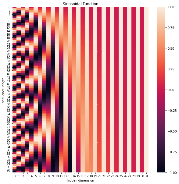
Here are the position embedding visualisations, you can find the pattern changes with the increasing embedding dimensions.
pe = PositionalEncoding(32, 0, 100)  # d_model, dropout-ratio, max_len
positional_encoding = pe.forward(Variable(torch.zeros(1, 100, 32))) # sequence length, d_model
plt.figure(figsize=(10,10))
sns.heatmap(positional_encoding.squeeze()) # 100x32 matrix
plt.title("Sinusoidal Function")
plt.xlabel("hidden dimension")
plt.ylabel("sequence length")
None
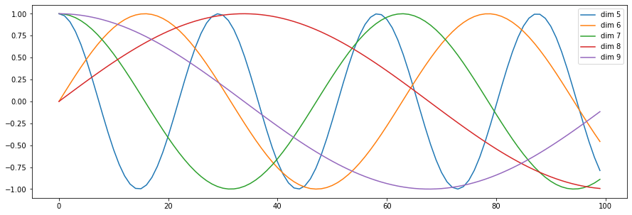
plt.figure(figsize=(15, 5))
pe = PositionalEncoding(24, 0)
y = pe.forward(Variable(torch.zeros(1, 100, 24)))
plt.plot(np.arange(100), y[0, :, 5:10].data.numpy())
plt.legend(["dim %d"%p for p in [5,6,7,8,9]])
None
2.2 Self Attention and Mask
An attention function can be described as mapping a query and a set of key-value pairs to an output, where the query, keys, values, and output are all vectors. The output is computed as a weighted sum of the values, where the weight assigned to each value is computed by a compatibility function of the query with the corresponding key.
We call our particular attention “Scaled-Dot-Product Attention”. The input consists of queries and keys of dimension dk, and values of dimension dv.
We compute the dot products of the query with all keys, divide each by square root of dk , and apply a softmax function to obtain the weights on the values.

The two most commonly used attention functions are additive attention, and dot-product (multiplicative) attention. Dot-product attention is identical to our algorithm, except for the scaling factor.
Additive attention computes the compatibility function using a feed-forward network with a single hidden layer. While the two are similar in theoretical complexity, dot-product attention is much faster and more space-efficient in practice, since it can be implemented using highly optimised matrix multiplication code.
To illustrate why the dot products get large, assume that the components of q and k are independent random variables with mean 0 and variance 1 . Then their dot product, 𝑞⋅𝑘q⋅k has mean 0 and variance dk, To counteract this effect, we scale the dot products by 1/sqrt(dk).
def attention(query, key, value, mask=None, dropout=None):
    "Compute 'Scaled Dot Product Attention'"
    d_k = query.size(-1)
    scores = torch.matmul(query, key.transpose(-2, -1)) / math.sqrt(d_k)
    if mask is not None:
        scores = scores.masked_fill(mask == 0, -1e9)
    p_attn = F.softmax(scores, dim=-1)
    if dropout is not None:
        p_attn = dropout(p_attn)
    return torch.matmul(p_attn, value), p_attn
Multi-head attention allows the model to jointly attend to information from different representation subspaces at different positions. With a single attention head, averaging inhibits this.
class MultiHeadedAttention(nn.Module):
    def __init__(self, h, d_model, dropout=0.1):
        "Take in model size and number of heads."
        super(MultiHeadedAttention, self).__init__()
        assert d_model % h == 0 # check the h number
        self.d_k = d_model // h
        self.h = h
        # 4 linear layers: WQ WK WV and final linear mapping WO
        self.linears = clones(nn.Linear(d_model, d_model), 4)
        self.attn = None
        self.dropout = nn.Dropout(p=dropout)

    def forward(self, query, key, value, mask=None):
        if mask is not None:
            # Same mask applied to all h heads.
            mask = mask.unsqueeze(1)
        nbatches = query.size(0) # get batch size
        # 1) Do all the linear projections in batch from d_model => h x d_k
        # parttion into h sections,switch 2,3 axis for computation.
        query, key, value = [l(x).view(nbatches, -1, self.h, self.d_k).transpose(1, 2)
                             for l, x in zip(self.linears, (query, key, value))]
        # 2) Apply attention on all the projected vectors in batch.
        x, self.attn = attention(query, key, value, mask=mask, dropout=self.dropout)
        # 3) "Concat" using a view and apply a final linear.
        x = x.transpose(1, 2).contiguous().view(nbatches, -1, self.h * self.d_k)
        return self.linears[-1](x) # final linear layer
Attention Mask
The input X is [batch−size, sequence−length], we use ‘padding’ to fill the matrix with 0 with respect to the longest sequence. But this will case issues for the softmax computation. This means the padding sections join the computation, but they shouldn’t. So we create this mask to ignore these area by assign a large negative bias. Thus, the masked area will lead to 0 so we avoid them in computation. We use mini-batch data as input, means we feed multiply lines of sentences into the model for training and computation.

In Transformer, both encoder and decoder attention computations need masking operation, but their functions are different. In the decoder, the self-attention layer is only allowed to attend to earlier positions in the output sequence. This is done by masking future positions (setting them to ‘-inf’) before the softmax step in the self-attention calculation.
The “Encoder-Decoder Attention” layer works just like multiheaded self-attention, except it creates its Queries matrix from the layer below it, and takes the Keys and Values matrix from the output of the encoder stack.
Here, we define a batch object that holds the src (English) and target sentences (Chinese) for training, as well as constructing the masks.
class Batch:
    "Object for holding a batch of data with mask during training."
    def __init__(self, src, trg=None, pad=0):
        # convert words id to long format.
        src = torch.from_numpy(src).to(DEVICE).long()
        trg = torch.from_numpy(trg).to(DEVICE).long()
        self.src = src
        # get the padding postion binary mask
        # change the matrix shape to  1×seq.length
        self.src_mask = (src != pad).unsqueeze(-2)
        # if target is not empty, mask decoder target.
        if trg is not None:
            # decoder input from target
            self.trg = trg[:, :-1]
            # decoder target from trg
            self.trg_y = trg[:, 1:]
            # add attention mask to decoder input
            self.trg_mask = self.make_std_mask(self.trg, pad)
            # check decoder output padding number
            self.ntokens = (self.trg_y != pad).data.sum()

    # Mask
    @staticmethod
    def make_std_mask(tgt, pad):
        "Create a mask to hide padding and future words."
        tgt_mask = (tgt != pad).unsqueeze(-2)
        tgt_mask = tgt_mask & Variable(subsequent_mask(tgt.size(-1)).type_as(tgt_mask.data))
        return tgt_mask # subsequent_mask is defined in 'decoder' section.
2.3 Layer Normalization and Residual Connection
1). LayerNorm:
Layer Normalization normalize the hidden layer output into standard format, i.i.d, to boost the training efficency and model weight convergence (row wise).
2). Residual Connection:
We employ a residual connection around each of the two sub-layers, followed by layer normalisation. We get the Value matrix with the weights from attentions Attention(Q,K,V), and then we transpose it to make sure it shares the same shape of X embedding.
class LayerNorm(nn.Module):
    def __init__(self, features, eps=1e-6):
        super(LayerNorm, self).__init__()
        self.a_2 = nn.Parameter(torch.ones(features))
        self.b_2 = nn.Parameter(torch.zeros(features))
        self.eps = eps

    def forward(self, x):
        mean = x.mean(-1, keepdim=True) # rows
        std = x.std(-1, keepdim=True)
        x_zscore = (x - mean)/ torch.sqrt(std ** 2 + self.eps)
        return self.a_2*x_zscore+self.b_2

class SublayerConnection(nn.Module):
    """
    A residual connection followed by a layer norm.
    Note for code simplicity the norm is first as opposed to last.
    SublayerConnection: connect Multi-Head Attention and Feed Forward Layers
    """
    def __init__(self, size, dropout):
        super(SublayerConnection, self).__init__()
        self.norm = LayerNorm(size)
        self.dropout = nn.Dropout(dropout)

    def forward(self, x, sublayer):
        "Apply residual connection to any sublayer with the same size."
        return x + self.dropout(sublayer(self.norm(x)))
2.4 Position-wise Feed-Forward Networks
In addition to attention sub-layers, each of the layers in our encoder and decoder contains a fully connected feed-forward network, which is applied to each position separately and identically. This consists of two linear transformations with a ReLU activation in between.
While the linear transformations are the same across different positions, they use different parameters from layer to layer. Another way of describing this is as two convolutions with kernel size 1.
class PositionwiseFeedForward(nn.Module):
    def __init__(self, d_model, d_ff, dropout=0.1):
        super(PositionwiseFeedForward, self).__init__()
        self.w_1 = nn.Linear(d_model, d_ff)
        self.w_2 = nn.Linear(d_ff, d_model)
        self.dropout = nn.Dropout(dropout)

    def forward(self, x):
        h1 = self.w_1(x)
        h2 = self.dropout(h1)
        return self.w_2(h2)
2.5 Transformer Encoder Overview
Now, we have programmed the four parts of the Transformer Encoder. Let us review how the data are transformed through all these layers.
- Word Embedding and Positional Encoding.
- Self-Attention and Mask.
- Residual Connection and Layer Normalization.
- Position-wise Feed-Forward Networks.
- Repeat 3.
def clones(module, N):
    """
    "Produce N identical layers. N=6 in the original paper."
    Use deepcopy the weight are indenpendent.
    """
    return nn.ModuleList([copy.deepcopy(module) for _ in range(N)])

class Encoder(nn.Module):
    "Core encoder is a stack of N layers (blocks)"
    def __init__(self, layer, N):
        super(Encoder, self).__init__()
        self.layers = clones(layer, N)
        self.norm = LayerNorm(layer.size)

    def forward(self, x, mask):
        """
        Pass the input (and mask) through each layer in turn.
        """
        for layer in self.layers:
            x = layer(x, mask)
        return self.norm(x)

# Each Encoder Block contains two sub-layers(Self-Attention,Position-wise) and 2 sublayer-connetions:
class EncoderLayer(nn.Module):
    def __init__(self, size, self_attn, feed_forward, dropout):
        super(EncoderLayer, self).__init__()
        self.self_attn = self_attn
        self.feed_forward = feed_forward
        self.sublayer = clones(SublayerConnection(size, dropout), 2)
        self.size = size # d_model

    def forward(self, x, mask):
        # X-embedding to Multi-head-Attention
        x = self.sublayer[0](x, lambda x: self.self_attn(x, x, x, mask))
        # X-embedding to feed-forwad nn
        return self.sublayer[1](x, self.feed_forward)
3. Decoder
After the introduction of the encoder structure, we can see the decoder shares a lot similarities of encoder.
It also stacks N times. But there is a Encoder-Deconder-Contex-Attention layer (sublayer[1]) between the Masked MHA[0] and FFN[2]. It use the output of the decoder as query to search the output of encoder with MHA, which makes decoder see all the outputs from encoder.
Decoding process:
- Input: Encoding output(memory) and i-1 position decoder output/
- Output: i position output work probabilities.
- decoding process works like RNN.

class Decoder(nn.Module):
    def __init__(self, layer, N):
        "Generic N layer decoder with masking."
        super(Decoder, self).__init__()
        self.layers = clones(layer, N)
        self.norm = LayerNorm(layer.size)

    def forward(self, x, memory, src_mask, tgt_mask):
        """
        Repeat decoder N times
        Decoderlayer get a input attention mask (src)
        and a output attention mask (tgt) + subsequent mask
        """
        for layer in self.layers:
            x = layer(x, memory, src_mask, tgt_mask)
        return self.norm(x)


class DecoderLayer(nn.Module):
    def __init__(self, size, self_attn, src_attn, feed_forward, dropout):
        super(DecoderLayer, self).__init__()
        self.size = size
        self.self_attn = self_attn
        self.src_attn = src_attn
        self.feed_forward = feed_forward
        self.sublayer = clones(SublayerConnection(size, dropout), 3)

    def forward(self, x, memory, src_mask, tgt_mask):
        m = memory # encoder output embedding
        x = self.sublayer[0](x, lambda x: self.self_attn(x, x, x, tgt_mask))
        x = self.sublayer[1](x, lambda x: self.src_attn(x, m, m, src_mask))
        # Context-Attention:q=decoder hidden,k,v from encoder hidden
        return self.sublayer[2](x, self.feed_forward)
We also modify the self-attention sub-layer in the decoder stack to prevent positions from attending to subsequent positions. This masking (subsequent_mask), combined with fact that the output embeddings are offset by one position, ensures that the predictions for position i can depend only on the known outputs at positions less than i .
For Encoder src-mask, just mask the padding cells.
But for decoder trg-mask, we need mask the padding and add the subsequent-mask process.
def subsequent_mask(size):
    "Mask out subsequent positions."
    attn_shape = (1, size, size)
    subsequent_mask = np.triu(np.ones(attn_shape), k=1).astype('uint8')
    return torch.from_numpy(subsequent_mask) == 0
Below the attention mask shows the position each tgt word (row) is allowed to look at (column). Words are blocked for attending to future words during training.”Yellow” color denote True.
plt.figure(figsize=(5,5))
plt.imshow(subsequent_mask(20)[0])
None

4. Transformer Model
Finally, let us put encoder and decoder together with the ‘generator’.
class Transformer(nn.Module):
    def __init__(self, encoder, decoder, src_embed, tgt_embed, generator):
        super(Transformer, self).__init__()
        self.encoder = encoder
        self.decoder = decoder
        self.src_embed = src_embed
        self.tgt_embed = tgt_embed
        self.generator = generator

    def encode(self, src, src_mask):
        return self.encoder(self.src_embed(src), src_mask)

    def decode(self, memory, src_mask, tgt, tgt_mask):
        return self.decoder(self.tgt_embed(tgt), memory, src_mask, tgt_mask)

    def forward(self, src, tgt, src_mask, tgt_mask):
        "Take in and process masked src and target sequences."
        # encoder output will be the decoder's memory for decoding
        return self.decode(self.encode(src, src_mask), src_mask, tgt, tgt_mask)

class Generator(nn.Module):
    def __init__(self, d_model, vocab):
        super(Generator, self).__init__()
        # decode: d_model to vocab mapping
        self.proj = nn.Linear(d_model, vocab)

    def forward(self, x):
        return F.log_softmax(self.proj(x), dim=-1)
Set Parameters and Create the Full Transformer model Function.
def make_model(src_vocab, tgt_vocab, N=6, d_model=512, d_ff=2048, h = 8, dropout=0.1):
    c = copy.deepcopy
    #  Attention
    attn = MultiHeadedAttention(h, d_model).to(DEVICE)
    #  FeedForward
    ff = PositionwiseFeedForward(d_model, d_ff, dropout).to(DEVICE)
    #  Positional Encoding
    position = PositionalEncoding(d_model, dropout).to(DEVICE)
    #  Transformer
    model = Transformer(
        Encoder(EncoderLayer(d_model, c(attn), c(ff), dropout).to(DEVICE), N).to(DEVICE),
        Decoder(DecoderLayer(d_model, c(attn), c(attn), c(ff), dropout).to(DEVICE), N).to(DEVICE),
        nn.Sequential(Embeddings(d_model, src_vocab).to(DEVICE), c(position)),
        nn.Sequential(Embeddings(d_model, tgt_vocab).to(DEVICE), c(position)),
        Generator(d_model, tgt_vocab)).to(DEVICE)

    # This was important from their code.
    # Initialize parameters with Glorot / fan_avg.
    # Paper title: Understanding the difficulty of training deep feedforward neural networks Xavier
    for p in model.parameters():
        if p.dim() > 1:
            nn.init.xavier_uniform_(p)
    return model.to(DEVICE)
5. Transformer Model Training: English-to-Chinese
Regularization Label Smoothing: During training, we employed label smoothing of value. This hurts perplexity, as the model learns to be more unsure, but improves accuracy and BLEU score.
class LabelSmoothing(nn.Module):
    "Implement label smoothing."
    def __init__(self, size, padding_idx, smoothing=0.0):
        super(LabelSmoothing, self).__init__()
        self.criterion = nn.KLDivLoss(reduction='sum') # 2020 update
        self.padding_idx = padding_idx
        self.confidence = 1.0 - smoothing
        self.smoothing = smoothing
        self.size = size
        self.true_dist = None

    def forward(self, x, target):
        assert x.size(1) == self.size
        true_dist = x.data.clone()
        true_dist.fill_(self.smoothing / (self.size - 2))
        true_dist.scatter_(1, target.data.unsqueeze(1), self.confidence)
        true_dist[:, self.padding_idx] = 0
        mask = torch.nonzero(target.data == self.padding_idx)
        if mask.dim() > 0:
            true_dist.index_fill_(0, mask.squeeze(), 0.0)
        self.true_dist = true_dist
        return self.criterion(x, Variable(true_dist, requires_grad=False))
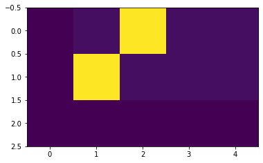
Here, ‘size’ is from vocabulary,’smoothing’ is value to be distributed on non-ground-truth. We can see an example of how the mass is distributed to the words based on confidence.
# Example of label smoothing.
crit = LabelSmoothing(5, 0, 0.1)  #  ϵ=0.4
predict = torch.FloatTensor([[0, 0.2, 0.7, 0.1, 0],
                             [0, 0.2, 0.7, 0.1, 0],
                             [0, 0.2, 0.7, 0.1, 0]])
v = crit(Variable(predict.log()), Variable(torch.LongTensor([2, 1, 0])))
# Show the target distributions expected by the system.
plt.imshow(crit.true_dist)
None
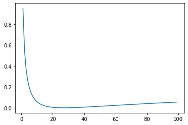
Label smoothing actually starts to penalize the model if it gets very confident about a given choice.]
crit = LabelSmoothing(5, 0, 0.1)
def loss(x):
    d = x + 3 * 1
    predict = torch.FloatTensor([[0, x / d, 1 / d, 1 / d, 1 / d]])
    return crit(Variable(predict.log()), Variable(torch.LongTensor([1]))).item()

plt.plot(np.arange(1, 100), [loss(x) for x in range(1, 100)])
None
Loss Computation
class SimpleLossCompute:
    def __init__(self, generator, criterion, opt=None):
        self.generator = generator
        self.criterion = criterion
        self.opt = opt

    def __call__(self, x, y, norm):
        x = self.generator(x)
        loss = self.criterion(x.contiguous().view(-1, x.size(-1)),
                              y.contiguous().view(-1)) / norm
        loss.backward()
        if self.opt is not None:
            self.opt.step()
            self.opt.optimizer.zero_grad()
        return loss.data.item() * norm.float()
Optimizer with Warmup Learning Rate
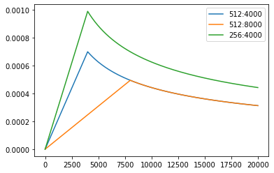
According to the paper, they applied a warmup learning rate with Adam Optimizer which updates the learning rate over the course of training. This corresponds to increasing the learning rate linearly for the first “warmup_steps” training steps, and decreasing it thereafter proportionally to the inverse square root of the step number.
class NoamOpt:
    "Optim wrapper that implements rate."
    def __init__(self, model_size, factor, warmup, optimizer):
        self.optimizer = optimizer
        self._step = 0
        self.warmup = warmup
        self.factor = factor
        self.model_size = model_size
        self._rate = 0

    def step(self):
        "Update parameters and rate"
        self._step += 1
        rate = self.rate()
        for p in self.optimizer.param_groups:
            p['lr'] = rate
        self._rate = rate
        self.optimizer.step()

    def rate(self, step = None):
        "Implement `lrate` above"
        if step is None:
            step = self._step
        return self.factor * (self.model_size ** (-0.5) * min(step ** (-0.5), step * self.warmup ** (-1.5)))

# We used factor=2, warmup-step = 4000
def get_std_opt(model):
    return NoamOpt(model.src_embed[0].d_model, 2, 4000,
            torch.optim.Adam(model.parameters(), lr=0, betas=(0.9, 0.98), eps=1e-9))
Example of the curves of this model for different model sizes and for optimization hyper-parameters.
# Three settings of the lrate hyperparameters.
opts = [NoamOpt(512, 1, 4000, None),
        NoamOpt(512, 1, 8000, None),
        NoamOpt(256, 1, 4000, None)]
plt.plot(np.arange(1, 20000), [[opt.rate(i) for opt in opts] for i in range(1, 20000)])
plt.legend(["512:4000", "512:8000", "256:4000"])
None
Training Iterators
def run_epoch(data, model, loss_compute, epoch):
    start = time.time()
    total_tokens = 0.
    total_loss = 0.
    tokens = 0.
    for i , batch in enumerate(data):
        out = model(batch.src, batch.trg, batch.src_mask, batch.trg_mask)
        loss = loss_compute(out, batch.trg_y, batch.ntokens)
        total_loss += loss
        total_tokens += batch.ntokens
        tokens += batch.ntokens
        if i % 50 == 1:
            elapsed = time.time() - start
            print("Epoch {:d} Batch: {:d} Loss: {:.4f} Tokens per Sec: {:.2f}s".format(epoch, i - 1, loss / batch.ntokens, (tokens.float() / elapsed / 1000.)))
            start = time.time()
            tokens = 0
    return total_loss / total_tokens

def train(data, model, criterion, optimizer):
    """
    Train and Save the model.
    """
    # init loss as a large value
    best_dev_loss = 1e5

    for epoch in range(EPOCHS):
        # Train model
        model.train()
        run_epoch(data.train_data, model, SimpleLossCompute(model.generator, criterion, optimizer), epoch)
        model.eval()

        # validate model on dev dataset
        print('>>>>> Evaluate')
        dev_loss = run_epoch(data.dev_data, model, SimpleLossCompute(model.generator, criterion, None), epoch)
        print('<<<<< Evaluate loss: {:.2f}'.format(dev_loss))

        # save the model with best-dev-loss (model validation)
        if dev_loss < best_dev_loss:
            best_dev_loss = dev_loss
            torch.save(model.state_dict(), SAVE_FILE) # SAVE_FILE = 'save/model.pt'
        print(f">>>>> current best loss: {best_dev_loss}")
Train and save the model
# Step 1: Data Preprocessing
data = PrepareData(TRAIN_FILE, DEV_FILE)
src_vocab = len(data.en_word_dict)
tgt_vocab = len(data.cn_word_dict)
print(f"src_vocab {src_vocab}")
print(f"tgt_vocab {tgt_vocab}")

# Step 2: Init model
model = make_model(
                    src_vocab,
                    tgt_vocab,
                    LAYERS,
                    D_MODEL,
                    D_FF,
                    H_NUM,
                    DROPOUT
                )

# Step 3: Training model
print(">>>>>>> start train")
train_start = time.time()
criterion = LabelSmoothing(tgt_vocab, padding_idx = 0, smoothing= 0.0)
optimizer = NoamOpt(D_MODEL, 1, 2000, torch.optim.Adam(model.parameters(), lr=0, betas=(0.9,0.98), eps=1e-9))

train(data, model, criterion, optimizer)
print(f"<<<<<<< finished train, cost {time.time()-train_start:.4f} seconds")
6. Prediction with English-to-Chinese Translator
def greedy_decode(model, src, src_mask, max_len, start_symbol):
    """
    Translate src with model
    """
    # decode the src
    memory = model.encode(src, src_mask)
    # init 1×1 tensor as prediction,fill in ('BOS')id, type: (LongTensor)
    ys = torch.ones(1, 1).fill_(start_symbol).type_as(src.data)
    #  run the length of the sentence
    for i in range(max_len-1):
        # decode one by one
        out = model.decode(memory,
                           src_mask,
                           Variable(ys),
                           Variable(subsequent_mask(ys.size(1)).type_as(src.data)))
        #  out to log_softmax
        prob = model.generator(out[:, -1])
        #  get the max-prob id
        _, next_word = torch.max(prob, dim = 1)
        next_word = next_word.data[0]
        #  concatenate with early predictions
        ys = torch.cat([ys,torch.ones(1, 1).type_as(src.data).fill_(next_word)], dim=1)
    return ys

def evaluate(data, model):
    """
    Make prediction with trained model, and print results.
    """
    with torch.no_grad():
        #  pick some random sentences from our data format.
        #  here I used 10 sentences from data.dev-en.
        #  you can easily modify this function from new input.
        for i in np.random.randint(len(data.dev_en), size=10):
            # Print English sentence
            en_sent = " ".join([data.en_index_dict[w] for w in data.dev_en[i]]) # space between English words
            print("\n" + en_sent)

            # Print Target Chinese sentence
            cn_sent =  " ".join([data.cn_index_dict[w] for w in data.dev_cn[i]]) # no space in Chinese words
            print("".join(cn_sent))

            # conver English to tensor
            src = torch.from_numpy(np.array(data.dev_en[i])).long().to(DEVICE)
            src = src.unsqueeze(0)
            # set attention mask
            src_mask = (src != 0).unsqueeze(-2)
            # apply model to decode, make prediction
            out = greedy_decode(model, src, src_mask, max_len=MAX_LENGTH, start_symbol=data.cn_word_dict["BOS"])
            # save all in the translation list
            translation = []
            # convert id to Chinese, skip 'BOS' 0.
            for j in range(1, out.size(1)):
                sym = data.cn_index_dict[out[0, j].item()]
                if sym != 'EOS':
                    translation.append(sym)
                else:
                    break
            print("translation: {}".format(" ".join(translation)))
English to Chinese Translator
# Predition
model.load_state_dict(torch.load(SAVE_FILE))
print(">>>>>>> start evaluate")
evaluate_start  = time.time()
evaluate(data, model)
print(f"<<<<<<< finished evaluate, cost {time.time()-
evaluate_start:.4f} seconds")
If your translation does not look good, that is totally OK. You can change the “Debug“ to False and retrain the model with CUDA support.
The following results are from my pertained model on Dell XPS15 with CUDA support. It took 1200s for 20 epoch on full dataset. I did not fine-tune the parameters, but you are welcomed to try.
# Here is my pretrained model with CUDA support
if DEVICE=="cuda":
    SAVE_FILE_EXTRA  = 'save/models/large_model.pt'
    model.load_state_dict(torch.load(SAVE_FILE_EXTRA))
    print(">>>>>>> start evaluate")
    evaluate_start  = time.time()
    evaluate(data, model)
    print(f"<<<<<<< finished evaluate, cost {time.time()-evaluate_start:.4f} seconds")
Model Input     : English Sentence, i.e., why do we work?
Model Target    : Chinese Sentence, i/e., 我 们 为 什 么 工 作?
Model Prediction: Translation from our Transformer Model in 中文.

>>>>>>> start evaluate
BOS i do n't feel like taking a walk this morning . EOS
BOS 我 今 天 早 上 不 想 散 步 。 EOS
translation: 我 今 天 不 想 去 散 步 。

BOS they go skiing at UNK every winter . EOS
BOS 他 們 每 年 冬 季 去 野 澤 滑 雪 。 EOS
translation: 他 們 每 年 去 滑 雪 。

BOS she greeted me with a smile . EOS
BOS 她 用 一 个 微 笑 迎 接 了 我 。 EOS
translation: 她 面 帶 微 笑 笑 笑 。

BOS i do n't expect that they will support my view . EOS
BOS 我 不 期 望 , 他 们 能 够 支 持 我 的 观 点 。 EOS
translation: 我 不 期 望 他 們 將 紅 色 的 。

BOS i ca n't take the place of her as an english teacher . EOS
BOS 我 无 法 取 代 她 做 英 语 老 师 。 EOS
translation: 我 不 能 忍 受 她 的 英 語 。

BOS why did you say such a thing ? EOS
BOS 你 為 什 麼 說 了 這 樣 的 事 ? EOS
translation: 你 為 什 麼 說 了 這 麼 這 麼 這 麼 這 麼 助 ?

BOS she was holding a small parasol in her hand . EOS
BOS 她 手 里 握 着 一 把 小 阳 伞 。 EOS
translation: 她 手 上 有 一 把 球 扔 。

BOS there was UNK any money left . EOS
BOS 几 乎 没 剩 下 钱 。 EOS
translation: 有 什 么 钱 就 在 来 一 下 来 。

BOS `` where were you ? '' `` i was at a friend 's house . '' EOS
BOS “ 你 在 哪 里 ? ” “ 我 在 一 个 朋 友 家 。 ” EOS
translation: “ 你 在 哪 里 ? ” “ 我 是 一 个 朋 友 ? ”

BOS he lost his eyesight in the accident . EOS
BOS 他 在 意 外 中 失 明 了 。 EOS
translation: 他 在 全 部 失 去 了 他 的 照 顾 生 。
<<<<<<< finished evaluate, cost 15.3620 seconds
All the data, source code and image on this page can be downloaded from my GitHub repository: https://github.com/cuicaihao/Annotated-Transformer-English-to-Chinese-Translator .
Download the pre-trained model file:
Reference
- The Annotated Transformer http://nlp.seas.harvard.edu/2018/04/03/attention.html
- The Illustrated Transformer http://jalammar.github.io/illustrated-transformer/
- GreedAI NLP Training Camp: https://www.greedyai.com/

Leave a comment